Why Is the GPU Still a Bottleneck? 为什么 GPU 还是瓶颈?
AI Infra Track Technology
This is the second note in my AI infrastructure learning series, following What Happens After a Prompt Enters an LLM? It is for readers who know the basics of large language models (LLMs) and want to understand the engineering limits. Numerical examples are teaching assumptions unless a source is given.
00 Picking Up the Previous Question
In Note 01, I learned why models need a key-value cache, or KV cache. It stores attention states so the model can reuse them while generating tokens. Requests with matching prefixes can also reuse compatible cached states.
But this creates a trade-off: saving computation takes memory, and GPU memory is finite.
Suppose I build an AI coding agent with an open-source 8B model. The model fits on the GPU. Why might the service still struggle when more users arrive?
Fitting the model into memory is only the first part of serving users.
I need to separate four questions. How much data can the GPU store? How fast can it move data? How much computation can it do? How does the service schedule competing requests?
01 What Uses GPU Memory?
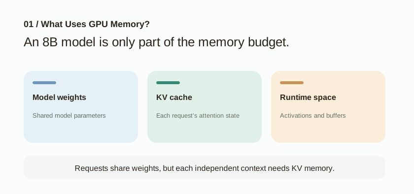
Start with model weights, the learned parameters. An 8B model has about eight billion parameters. BF16, a 16-bit number format, uses 2 bytes per parameter. The weights alone take about 16 billion bytes, or 14.9 GiB.
The GPU also needs KV cache for active requests. It must leave room for activations, the intermediate values computed by the model, along with temporary buffers and other runtime data.
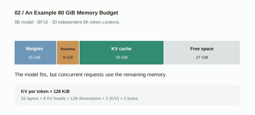
Suppose the service has 80 GiB of usable memory. Weights take 15 GiB and runtime data takes 8 GiB. Thirty independent requests each need about 1 GiB of KV cache. Total use is 15 + 8 + 30 = 53 GiB, leaving 27 GiB. Subtracting the weights alone would suggest 65 GiB free and miss most of the request memory.
Why would one request need 1 GiB of KV cache?
That amount depends on the model. Suppose it has 32 transformer layers, 8 KV heads per layer, and 128 dimensions per head. With BF16 cache values, KV memory per token is approximately:
The first 2 counts the key and value states. The last 2 is the number of bytes per BF16 value. An 8,192-token context therefore needs about 1 GiB of KV cache.
These dimensions match common Llama 8B configurations. Other models, number formats, and attention designs can have very different memory needs.
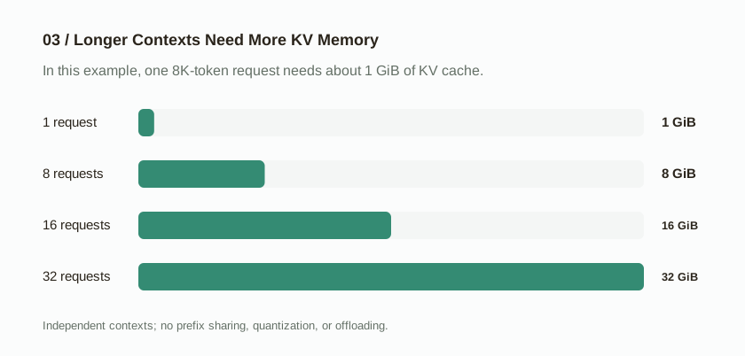
The distinction I had missed was simple: requests on one model instance share weights, but independent contexts need additional KV cache. Matching prefixes may share some cached states. I cannot assume that every user sends the same context.
Could we just shorten the context?
That was my first idea. A coding agent could drop older messages or send fewer repository files. This saves memory, but it might remove information the model needs to understand dependencies between files.
Another option is to keep the context and use prefix caching. This helps when many requests share the same beginning. If users work in different repositories, they may share little project context. A single user may reuse context across turns, but the cache still has a capacity limit.
A service can combine context selection, prefix reuse, and cache eviction, which discards cached states to free space. I would judge that combination by model usefulness and user experience within the memory budget. Cache hit rate alone is too narrow a goal.
02 Capacity, Bandwidth, and Compute
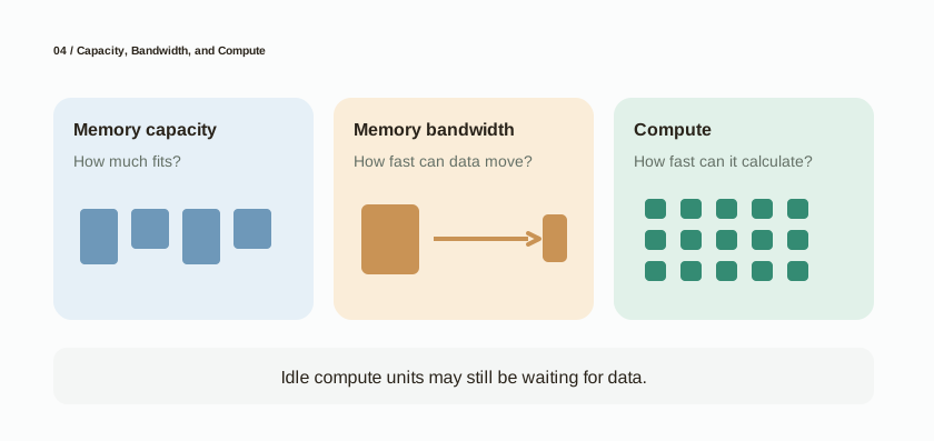
When I started learning about GPUs, memory capacity, memory bandwidth, and compute throughput sounded similar. They describe different limits.
| Resource | Question | Common Unit |
|---|---|---|
| Memory capacity | Can the model and request states fit at the same time? | GiB |
| Memory bandwidth | How fast can data move to and from GPU memory? | GB/s, TB/s |
| Compute throughput | How many mathematical operations can the hardware do per second? | FLOP/s |
A GPU can slow down while waiting for data even if it has free memory. Adding more compute units does little for a workload that is already waiting on memory bandwidth.
Suppose one decode step with a small batch reads about 16 GB of weights from memory. At an effective bandwidth of 1 TB/s, moving those bytes alone takes at least about 16 ms under idealized conditions.
This is not a prediction of end-to-end generation time. It leaves out caching, computation, KV access, and other costs. The calculation shows how data movement can set a lower bound on execution time.
Why do prefill and decode have different bottlenecks?
Prefill processes the input tokens. Their positions are already known, so the model can compute many positions together and reuse weights across them. With a large input, compute speed often limits this stage.
Decode generates the output. A standard autoregressive model usually generates one new token per request at each step. With a small batch, that step reads a lot of model data for relatively little computation. Memory bandwidth often becomes the limit.
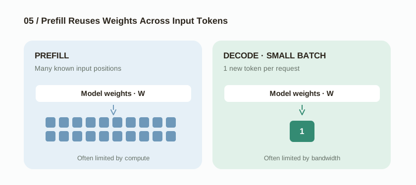
Arithmetic intensity measures how many mathematical operations happen per byte moved.
Higher arithmetic intensity gives compute units more work for each byte read. With low intensity, the GPU may spend more time waiting for data.
These are common patterns, not fixed rules. The model, batch size, context length, GPU computation routines called kernels, and hardware all affect the bottleneck.
03 Why can a larger batch slow down each user?
I kept returning to this question. Batching improves GPU efficiency, so I initially expected every user to get an answer faster. But total work and individual waiting time measure different things.
For a linear layer, computing one token can be written as y = xW. Stacking token representations from different requests into a matrix X gives Y = XW. The weights W now serve more computation together.
This can raise total throughput, the amount of work the service completes per second. A larger batched step still does more work than a small one, so it may take longer even while producing more tokens.
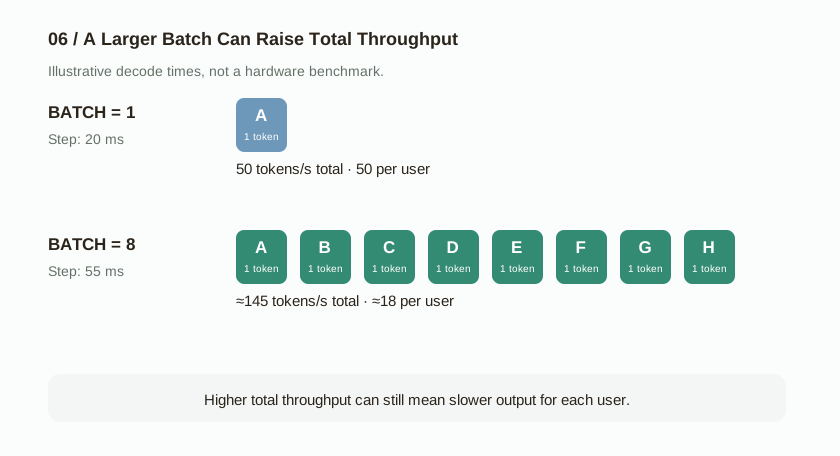
| Metric | Batch 1 | Batch 8 |
|---|---|---|
| One decode step | 20 ms | 55 ms |
| Total tokens per step | 1 token | 8 tokens |
| Total throughput | 50 tokens/s | ≈145 tokens/s |
| Output rate per user | 50 tokens/s | ≈18 tokens/s |
In the eight-user batch, each user receives one token in 55 ms. Each does not receive eight tokens. The service produces more tokens overall, but the gap between each user's tokens grows from 20 ms to 55 ms.
This is a latency-throughput trade-off. It does not mean every increase in batch size makes users slower. If the GPU has spare resources, a larger batch may barely increase step time. The result depends on when compute, bandwidth, memory, or scheduling becomes the limit.
Three Metrics to Keep Separate
| Metric | What It Measures |
|---|---|
| TTFT | Time to first token: how long the user waits for the first output token, including queueing and other stages. |
| ITL / TPOT | Inter-token latency / time per output token: gaps between output tokens or average time per output token. Benchmark definitions differ. |
| Throughput | The whole service's work per second, such as output tokens/s. |
These metrics answer different business questions. A high-volume model API may prioritize throughput and cost per token. An interactive coding assistant may prioritize TTFT and smooth streaming.
If throughput rises by 40% while user latency stays about the same, some customers benefit. Calling that result “40% faster answers” would misrepresent what changed.
04 Requests Start and Finish at Different Times
Real traffic adds another complication. User A needs 2,000 output tokens, B needs 100, and C needs 500. D arrives later.
If a fixed batch must finish together, resources may sit idle after short requests finish. D may wait for A, the longest request. Continuous batching lets the scheduler remove finished requests and admit new ones between generation steps.
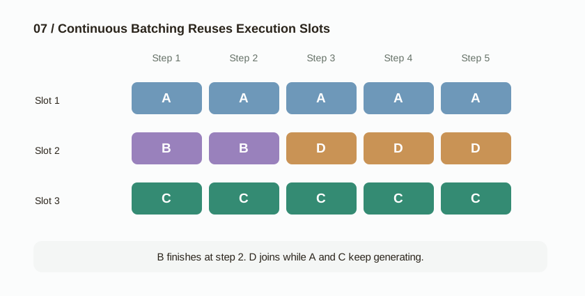
The scheduler has to track more than arrival order. Every active request uses KV memory. Some requests are in prefill; others are decoding. Admitting, pausing, and removing requests changes the available resources.
Continuous batching gives the GPU more chances to do useful work. Capacity and bandwidth still limit it. When demand is high enough, the scheduler must choose which work runs first.
05 Why can a long prefill interrupt decode?
Return to the coding agent. At 9 a.m., many developers send prompts containing large repositories. Other users already have answers streaming back.
If prefill and decode share the same GPU workers, a long prefill can occupy execution resources and pause those answers. A delay that looks like a network problem may come from GPU scheduling.
Option A: Chunked Prefill
Chunked prefill splits a large prompt into smaller pieces. The scheduler can run decode between chunks. Some implementations also mix prefill and decode work in one iteration.
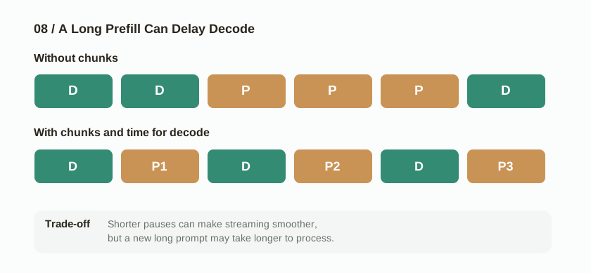
This can shorten pauses between output tokens. Processing a new prompt may take longer, raising TTFT. Results depend on chunk size, scheduling policy, and workload. This approach usually needs fewer architectural changes than separating GPU worker pools.
Option B: Prefill-Decode Disaggregation
Prefill-decode disaggregation runs the two stages on different GPU workers or resource pools. Prefill workers process the input context. Decode workers generate output tokens. After prefill, the service transfers the KV cache needed for generation to the decode workers.
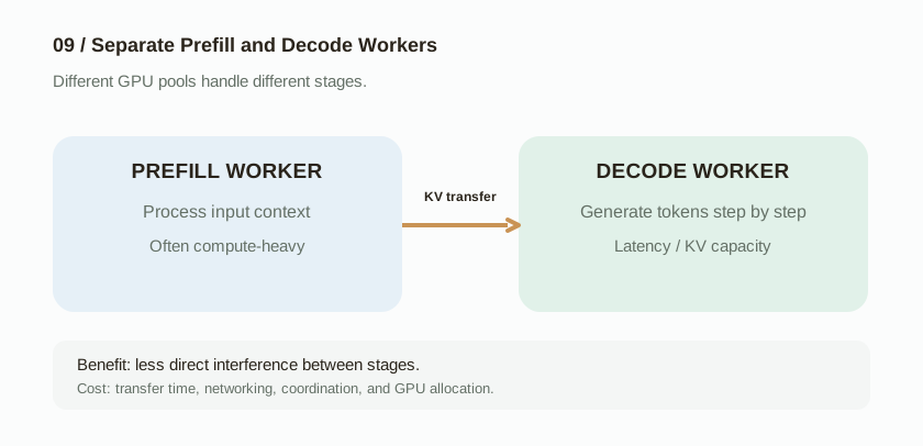
Separating the workers can reduce direct interference between long prefills and ongoing decode. But KV transfer takes time and network bandwidth. Long prompts can create large caches. The service also needs more routing, resource allocation, and operational work.
Separate pools can also cost more. At light load, a shared worker may be simpler and avoid transfers between workers. Dedicated pools may offer more value under sustained, heavy traffic that mixes prefill and decode.
06 How would I choose as a product manager?
I first noticed two costs: chunking may delay the completion of a new prefill, while separate pools add KV transfers and deployment complexity. That is a start, but it is too little for a product decision.
I would first ask: what are users waiting for? Is the first token late? Does output pause midway? Are requests stuck in a queue? Then I would inspect traffic during the problem, rather than rely on averages for the whole day.
Inspect the Workload
Input and output lengths, morning traffic peaks, concurrent requests, cache hits, and queue length.
Find the Bottleneck
Compute, high-bandwidth memory (HBM) bandwidth, KV memory, network transfer, or scheduling interference.
Compare Trade-offs
p95/p99 TTFT and ITL, completed requests, GPU cost, reliability, and complexity.
Test the User Goal
Replay representative requests and compare the options at similar cost.
I would compare the current system, chunked prefill, separate pools, and a combination if needed. With one GPU pool and brief daily peaks, chunking may be the practical first test. If large prefills constantly interrupt decode, separate pools deserve testing, provided KV transfer is fast enough.
For complaints about output freezing, I would pay particular attention to p95 and p99 ITL. The p95 value covers 95% of measured intervals; p99 covers 99%. These percentiles show the slower end of the distribution. A low average can hide pauses that make the product frustrating to use.
07 From System Metrics to User Value
I now ask three questions about an optimization: which workload does it help, which bottleneck does it reduce, and what does it cost?
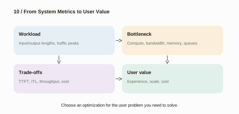
Suppose an engineer says, “Our change raises throughput by 40%, but latency for each user stays about the same.”
For a high-volume inference API, the same GPUs may now do more work. With enough demand, that could lower infrastructure cost per token.
For an interactive coding assistant whose users complain about pauses, the result does not show that output feels faster. It may still help the company serve more users without GPU costs growing at the same rate. That is a separate benefit to measure.
An optimization can be technically effective and still leave a particular customer's main problem unsolved.
Understand the workload, find the bottleneck, compare the costs, and measure the result users care about.
08 Connecting the Ideas
I now ask five questions about GPU performance. Does the state fit? How must data move? Which computations dominate? How do requests interfere? Which result matters to the user?
The same coding agent may need different architectures as traffic changes. I would keep measuring, comparing, and adjusting as its workload grows.
The diagrams, batch timings, and memory budgets explain mechanisms. They are not official architectures or measured benchmarks. Actual results depend on model design, numerical precision, GPU links, kernels, concurrency, and scheduling policy.
Further Reading and References
- TNG Technology: Prefill and Decode for Concurrent Requests: The compute and bandwidth patterns of prefill and decode.
- NVIDIA TensorRT-LLM: Disaggregated Serving: Why separate prefill and decode.
- NVIDIA Dynamo: Disaggregated Serving: KV transfer and resource allocation trade-offs.
- vLLM: Architecture Overview and Scheduler: An example of scheduling in an open-source inference engine.
- Kwon et al. (2023): PagedAttention: KV cache memory management.
- Llama 3.1 8B Configuration Example: The model dimensions used in the KV cache estimate.
这是我 AI 基础设施学习系列的第二篇,接在 提示词进了 LLM 之后发生了什么? 后面。写给已经知道大语言模型(LLM)基础、想看懂工程上限的人。数字如果没有给出处,就是为了讲清楚而设的假设。
00 接着上一个问题
在笔记 01 里,我搞懂了模型为什么需要键值缓存,也就是 KV cache。它存着 attention 的状态,生成 token 时可以复用。前缀相同的请求,也可以复用彼此兼容的缓存。
但这里有个取舍:省下计算,要用掉显存,而 GPU 显存是有限的。
假设我用一个开源的 8B 模型做 AI 编程助手。模型放得进 GPU。用户一多,服务为什么还是会吃力?
模型放进显存,只是服务用户的第一步。
我得把四个问题分开。GPU 能存多少数据?数据搬得有多快?计算做得了多少?服务怎么安排互相抢资源的请求?
01 GPU 显存被什么占着?
先看模型权重,也就是学出来的参数。一个 8B 模型大约有八十亿个参数。BF16 是一种 16 位的数字格式,每个参数 2 字节。光是权重就要大约 160 亿字节,也就是 14.9 GiB。
GPU 还要给正在处理的请求留 KV cache。激活值(模型算到一半的中间结果)、临时缓冲和其他运行时数据,也得留地方。
假设服务有 80 GiB 可用显存。权重占 15 GiB,运行时数据占 8 GiB。30 个互不相干的请求,每个大约要 1 GiB 的 KV cache。一共是 15 + 8 + 30 = 53 GiB,还剩 27 GiB。如果只减掉权重,会以为还空着 65 GiB,请求真正占的显存大部分就被漏掉了。
一个请求为什么会要 1 GiB 的 KV cache?
这个数取决于模型。假设它有 32 层 transformer,每层 8 个 KV head,每个 head 128 维。缓存值用 BF16 时,每个 token 的 KV 显存大约是:
第一个 2 是 key 和 value 两份状态。最后一个 2 是每个 BF16 数值占的字节。所以 8,192 个 token 的上下文,大约需要 1 GiB 的 KV cache。
这些尺寸和常见的 Llama 8B 配置对得上。别的模型、数字格式和 attention 设计,显存可以差很多。
我之前没分开的一点其实很简单:同一个模型实例上的请求共用权重,但互不相干的上下文要各自再占一份 KV cache。前缀相同的可以共用一部分缓存。不能假设每个用户发来的上下文都一样。
把上下文截短就行了吗?
这是我的第一个想法。编程助手可以丢掉更早的消息,或者少传一些仓库文件。显存是省了,但模型看文件之间依赖时需要的信息,也可能被丢掉。
另一种做法是保留上下文,用前缀缓存。很多请求开头相同时,这有用。如果用户在不同的仓库里工作,能共用的项目上下文可能很少。同一个用户在多轮对话里可以复用上下文,但缓存本身还有容量上限。
服务可以把三件事合在一起:挑选上下文、复用前缀、以及在空间不够时丢掉缓存状态。我会用显存预算之内的模型是否还有用、用户体验如何来判断这套组合。只看缓存命中率,目标太窄了。
02 容量、带宽和计算
我刚开始学 GPU 的时候,显存容量、显存带宽和计算吞吐听起来差不多。它们说的是不同的上限。
| 资源 | 问题 | 常见单位 |
|---|---|---|
| 显存容量 | 模型和请求状态能不能同时放进去? | GiB |
| 显存带宽 | 数据在 GPU 显存之间来回搬,能有多快? | GB/s、TB/s |
| 计算吞吐 | 硬件每秒能做多少次数学运算? | FLOP/s |
显存还有空,GPU 也可能因为在等数据而慢下来。负载已经卡在显存带宽上时,再加计算单元用处不大。
假设 batch 很小的时候,一次 decode 要从显存里读大约 16 GB 的权重。有效带宽 1 TB/s 时,光是把这些字节搬完,理想情况下至少大约要 16 毫秒。
这不是在预测端到端的生成时间。缓存、计算、读取 KV 和其他开销都没算进去。这个计算只说明:数据搬运可以给执行时间设一条下限。
为什么 prefill 和 decode 的瓶颈不一样?
Prefill 处理输入 token。它们的位置已经知道,所以模型可以一次算很多个位置,并在这些位置之间复用权重。输入很长时,这一段常常卡在计算速度上。
Decode 生成输出。标准的自回归模型,每个请求每一步通常只新生成一个 token。batch 小时,这一步为了相对很少的计算,要读很多模型数据。上限常常变成显存带宽。
算术强度衡量每搬一个字节,做了多少次数学运算。
算术强度高,计算单元每读一个字节就有更多活干。强度低的时候,GPU 可能把更多时间花在等数据上。
这是常见的情况,不是固定规则。模型、batch 大小、上下文长度、GPU 上实际跑的计算例程(kernel),还有硬件,都会影响瓶颈在哪。
03 为什么 batch 变大,每个用户会变慢?
这个问题我反复回来看。Batching 能让 GPU 更忙,所以我一开始以为每个用户都会更快拿到回答。但系统一共干了多少活,和一个人等了多久,是两件事。
对一个线性层,算一个 token 可以写成 y = xW。把不同请求的 token 表示叠成矩阵 X,就变成 Y = XW。权重 W 这一次服务了更多计算。
这可以提高总吞吐,也就是服务每秒完成的工作量。更大的 batch 这一步干的活仍然比小 batch 多,所以即便吐出的 token 更多,这一步也可能更久。
| 指标 | Batch 1 | Batch 8 |
|---|---|---|
| 一次 decode | 20 ms | 55 ms |
| 每步的 token 总数 | 1 个 token | 8 个 token |
| 总吞吐 | 50 token/s | 约 145 token/s |
| 每个用户的输出速度 | 50 token/s | 约 18 token/s |
八个用户的 batch 里,每个人是 55 毫秒拿到一个 token。不是一个人拿到八个 token。服务整体产出的 token 更多了,但同一个用户前后两个 token 的间隔,从 20 毫秒变成了 55 毫秒。
这是延迟和吞吐的取舍。不是说 batch 变大就一定让用户更慢。GPU 还有余量时,batch 大一点,这一步的时间可能几乎不变。结果取决于上限先出现在计算、带宽、显存,还是调度上。
三个要分开看的指标
| 指标 | 它量的是什么 |
|---|---|
| TTFT | 首 token 时间:用户等到第一个输出 token 的时间,包括排队和其他阶段。 |
| ITL / TPOT | token 间隔 / 每个输出 token 的时间:输出 token 之间的空隙,或者每个输出 token 的平均时间。Benchmark 的定义并不统一。 |
| 吞吐 | 整个服务每秒干的活,比如每秒输出多少 token。 |
这些指标回答的是不同的业务问题。量大的模型 API 可能优先看吞吐和每个 token 的成本。交互式的编程助手可能优先看 TTFT,以及流式输出顺不顺。
如果吞吐提高了 40%,用户延迟差不多没变,有些客户会受益。把这个结果说成“回答快了 40%”,说的就不是实际变了的那件事。
04 请求开始和结束的时间不一样
真实流量还更麻烦。用户 A 要 2,000 个输出 token,B 要 100 个,C 要 500 个。D 晚一点才来。
如果一个固定的 batch 必须一起结束,短请求结束后,资源可能空着。D 可能得等最长的那个请求 A。 连续 batching 让调度器在生成的步骤之间拿走已经结束的请求,再放进新的。
调度器要盯的不只是谁先到。每个还在跑的请求都占 KV 显存。有的请求在 prefill,有的在 decode。放进、暂停、拿走请求,都会改变还剩多少资源。
连续 batching 让 GPU 有更多机会去干有用的活。容量和带宽仍然限制着它。需求够高时,调度器必须选择先跑哪一份工作。
05 为什么很长的 prefill 会打断 decode?
回到编程助手。早上 9 点,很多开发者发来带着大仓库的提示词。另一些用户的回答已经在往外流。
如果 prefill 和 decode 共用同一批 GPU worker,一段很长的 prefill 会占住执行资源,把那些正在输出的回答按住。看起来像网络问题的卡顿,可能来自 GPU 调度。
做法 A:分块 prefill
分块 prefill 把很长的提示词切成小块。调度器可以在块和块之间跑 decode。有的实现还会在同一次迭代里把 prefill 和 decode 混在一起。
输出 token 之间的停顿可以变短。新提示词处理完可能更久,TTFT 会上去。结果取决于块有多大、调度策略是什么、负载是什么。和把 GPU worker 拆成不同的池相比,这种做法通常要改的架构更少。
做法 B:Prefill 和 decode 拆开
Prefill-decode 分离是把两个阶段放在不同的 GPU worker 或资源池上。Prefill 的 worker 处理输入上下文。Decode 的 worker 生成输出 token。Prefill 结束后,服务把生成所需要的 KV cache 传给 decode 的 worker。
把 worker 分开,可以减少长 prefill 和正在进行的 decode 直接互相打扰。但 传 KV 要时间和网络带宽。长提示词会造出很大的缓存。服务还得做更多路由、资源分配和运维。
分开的池也可能更贵。负载轻的时候,共用一个 worker 可能更简单,也省掉 worker 之间的传输。持续、很重、而且 prefill 和 decode 混在一起的流量下,专用的池可能更值。
06 如果我是产品经理,会怎么选?
我先看见两笔成本:切块可能让一次新的 prefill 更晚做完;分开的池则多了 KV 传输和部署上的复杂度。这是个开头,但拿来做产品决定还太少。
我会先问:用户在等什么?是第一个 token 来得晚?是输出到一半停住?还是请求卡在队列里?然后我会去看出问题那段时间的流量,而不是拿一整天的平均数来判断。
看负载
输入和输出有多长、早高峰、同时有多少请求、缓存命中、队列有多长。
找瓶颈
计算、高带宽显存(HBM)的带宽、KV 显存、网络传输,还是调度上的互相干扰。
比取舍
p95 / p99 的 TTFT 和 ITL、完成了多少请求、GPU 成本、稳定性,以及复杂度。
按用户的目标来测
重放有代表性的请求,在差不多的成本下比较这几个选项。
我会比现在的系统、分块 prefill、分开的池,必要的话再加上组合。如果只有一个 GPU 池,而且每天的高峰很短,切块可能是第一个值得试的。如果大的 prefill 一直在打断 decode,分开的池值得测,前提是 KV 传得够快。
如果抱怨的是输出卡住,我会特别看 p95 和 p99 的 ITL。p95 覆盖 95% 的测量间隔,p99 覆盖 99%。这两个分位数看的是分布里慢的那一头。平均数很低,也可以藏住让产品用起来很烦的停顿。
07 从系统指标到用户在乎的事
现在看一项优化,我会问三个问题:它帮的是哪种负载,它减轻的是哪个瓶颈,它要付出什么。
假设一个工程师说:“我们的改动把吞吐提高了 40%,但每个用户的延迟差不多没变。”
对一个量大的推理 API,同样的 GPU 现在可能干更多活。需求够的话,每个 token 的基础设施成本可以降下来。
对一个交互式的编程助手,用户抱怨的是停顿,这个结果并不能说明输出感觉更快了。它仍然可能帮公司在 GPU 成本没有同比上涨的情况下服务更多用户。那是另一笔要单独去量的好处。
一项优化可以在技术上有效,同时仍然没有解决某个客户最主要的问题。
看清负载,找到瓶颈,把成本比一比,再去量用户在乎的那个结果。
08 把这些想法串起来
现在看 GPU 性能,我会问五个问题。状态放得下吗?数据必须怎么搬?哪些计算占大头?请求之间怎么互相影响?哪个结果是用户在乎的?
同一个编程助手,流量变了,需要的架构也可能变。负载长大的时候,我会继续测、继续比、继续调。
图、batch 的时间和显存预算是用来解释机制的。它们不是官方架构,也不是测出来的 benchmark。实际结果取决于模型设计、数值精度、GPU 之间的连接、kernel、并发和调度策略。
延伸阅读和参考
- TNG Technology:并发请求下的 Prefill 和 Decode:prefill 和 decode 在计算和带宽上的不同表现。
- NVIDIA TensorRT-LLM:分离式服务:为什么把 prefill 和 decode 分开。
- NVIDIA Dynamo:分离式服务:KV 传输和资源分配上的取舍。
- vLLM:架构概览和调度器:开源推理引擎里调度长什么样的一个例子。
- Kwon 等人(2023):PagedAttention:KV cache 的显存管理。
- Llama 3.1 8B 配置示例:估算 KV cache 时用到的模型尺寸。